Genuary 2025 - 2 Layers upon layers upon layers
2025 February 16
1 minute read
#creative coding
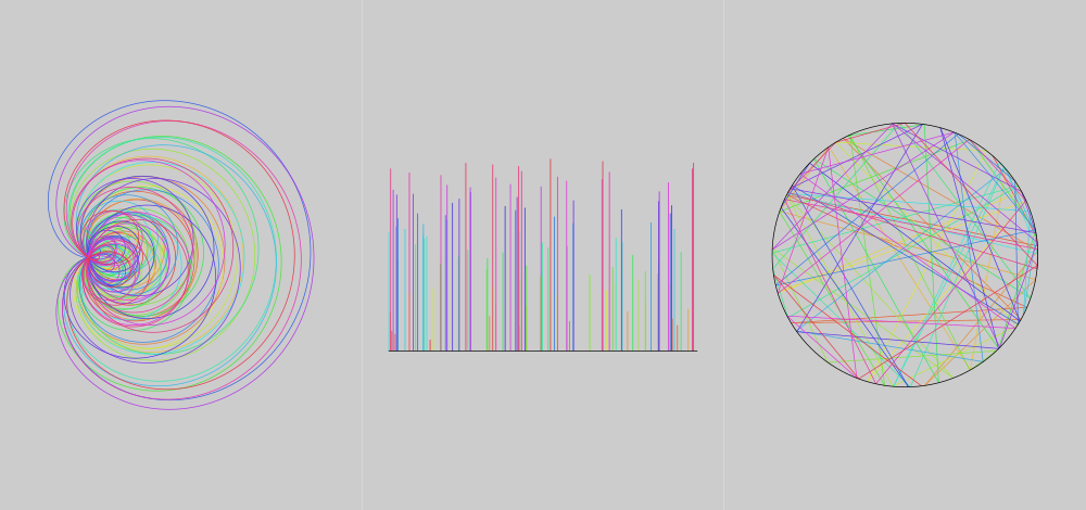
p5 sketch for Genuary day 2.
p5 sketch for Genuary day 2.
p5 sketch for Genuary day 1.
Learning p5
First created in nannou
A ray tracer based on the raytracer construction kit by matklad.
I focused mostly on not relying on any third party crates with this project. Building up mini libraries for geometry, colors, image creation and then of course the ray tracer itself. I stopped at the point where it suggests to make a mini language for scene description files as I've never done anything like that before. So I decided I would go do that separately first.

By combining introduction to nannou in the tutorial and the Coding train loop tutorial I created Cube Schotter.
By combining introduction to nannou in the tutorial and the Coding train loop tutorial I created schotter5.
Based on tsulej's article, I recreated the rendering engine with nannou.
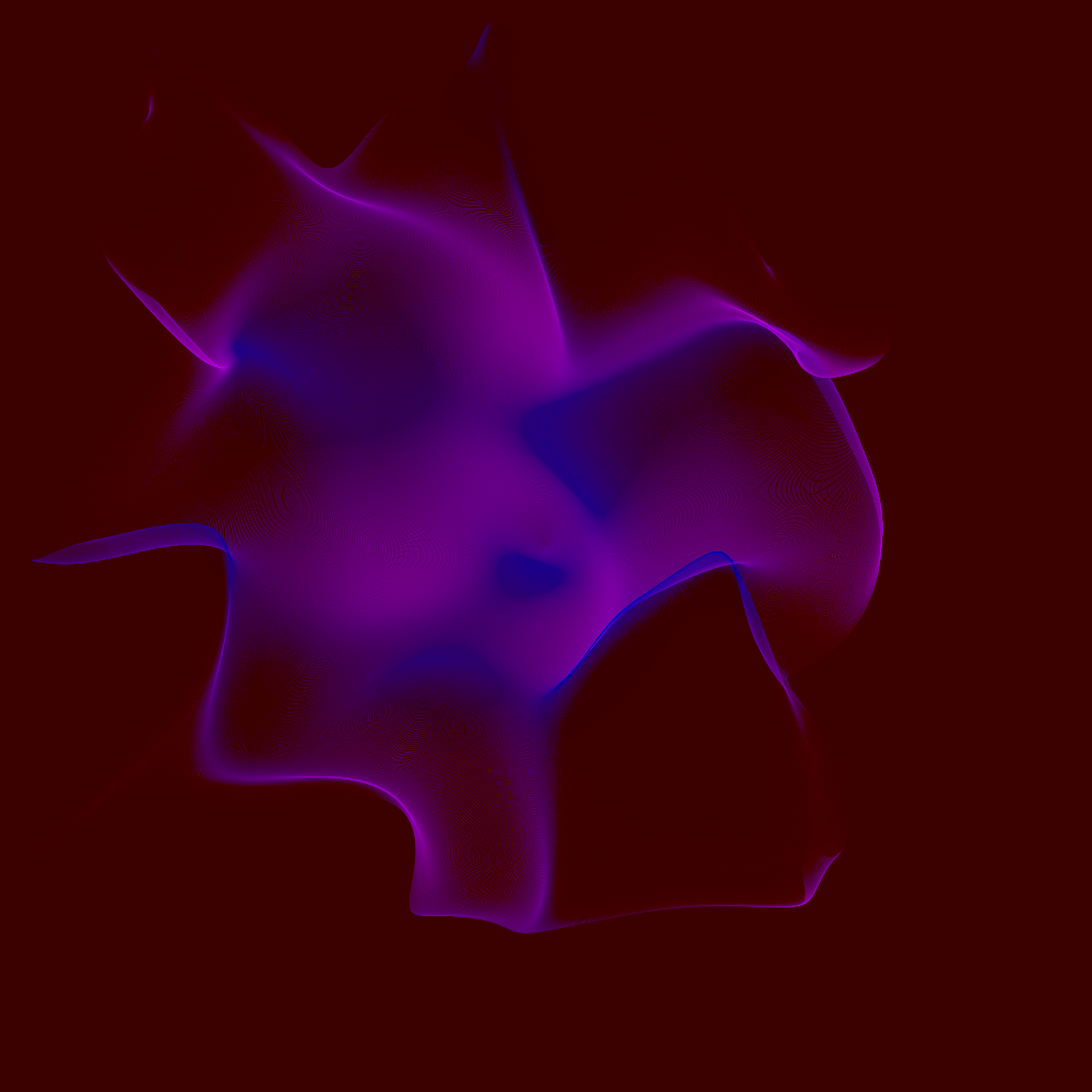 My purple version of tsulej's pictures.
Which uses the normal distribution as a random source.
fn expectation(xy: Vec2) -> f32 {
    (-xy.length().pow(2.0) / 2.0).exp()
}
And a mapping to color and position via:
    let r = point_param.noise_scale * xy.length();
    let t = vec2(
        (noise.get([xy.x as f64, xy.y as f64, point_param.noise_pos.x.into()]) - 0.5) as f32,
        (noise.get([
            (xy.y - 1.1) as f64,
            (xy.x + 1.1) as f64,
            point_param.noise_pos.y.into(),
        ]) - 0.5) as f32,
    );
    let nxy = r * t;
    (
        point_param.zero_point + point_param.scale * xy + nxy,
        basic_color(lerp_colors(colors, t.length())),
    )
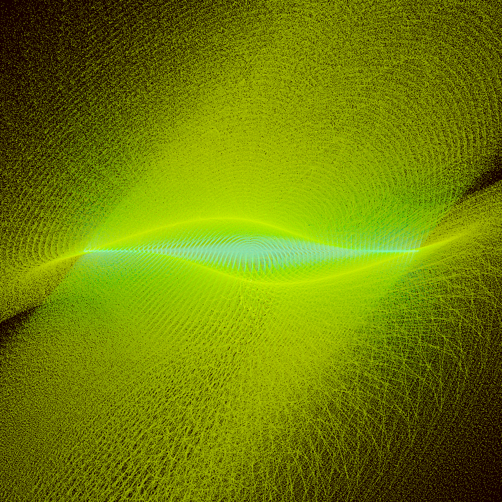 Using a random distribution of
(-xy.length().sin().pow(2.0) / 2.0).exp()
And a generation of
    let r = point_param.noise_scale * xy.length();
    let psi = r * xy.angle();
    let t = xy.x
        * vec2(
            (psi + point_param.noise_pos.x).cos() + (psi + point_param.noise_pos.x).sin(),
            (psi + point_param.noise_pos.y).cos() - (psi + point_param.noise_pos.y).sin(),
        );
    let nxy = r * t;
    (
        point_param.zero_point + point_param.scale * xy + nxy,
        basic_color(lerp_colors(colors, t.length())),
    )
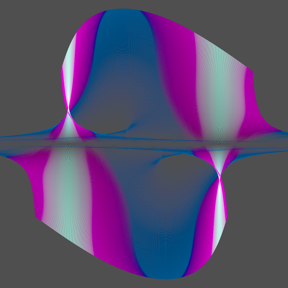 Using a random distribution of
1.0 - (-xy.length().pow(2.0) / 2.0).exp()
And a generation of
    let r = point_param.noise_scale * xy.length();
    let t = vec2(xy.x.sin() * xy.y.cos() as f32, xy.y.cos() / xy.x);
    let nxy = r * t;
    (
        point_param.zero_point + point_param.scale * xy + nxy,
        basic_color(lerp_colors(colors, t.length())),
    )
You can see it's easy to make new images by combining different transcendental functions.
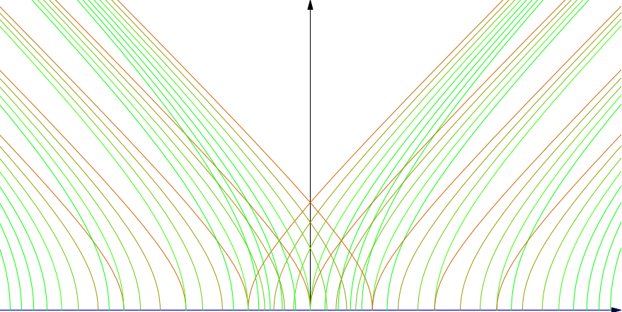
I found another couple of interesting images from my masters.
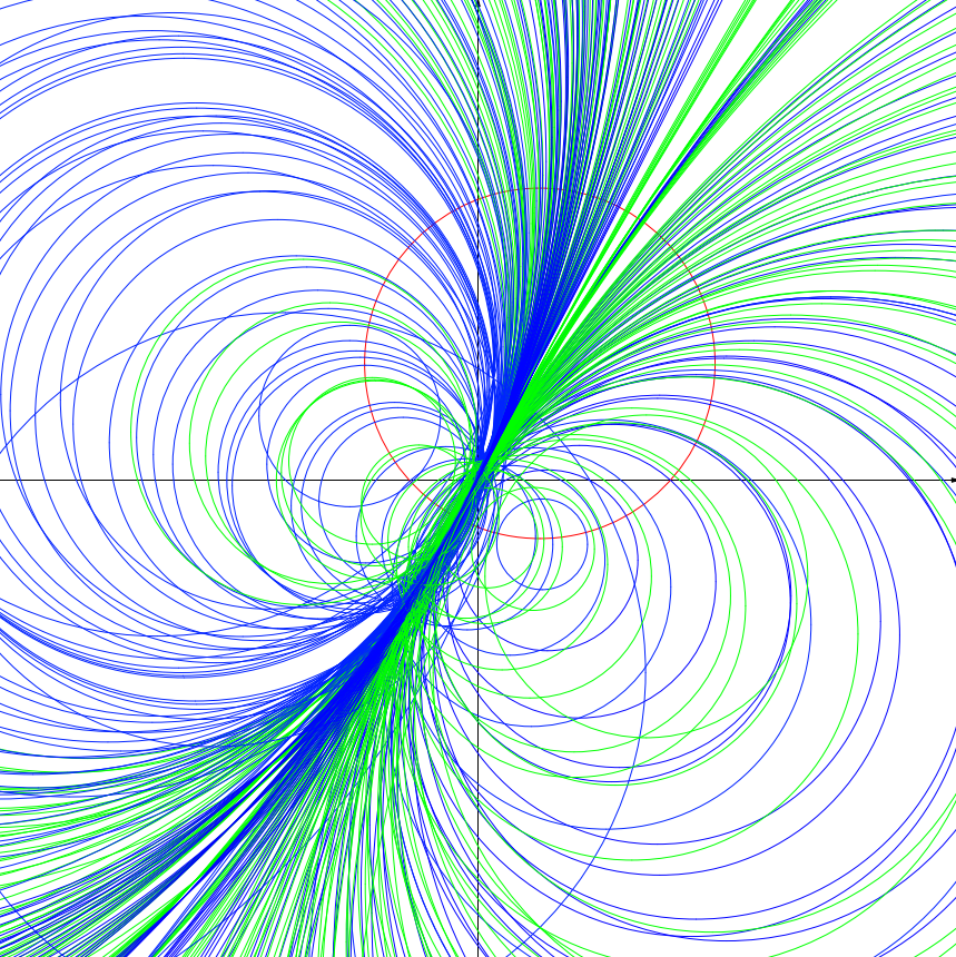
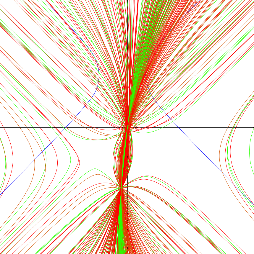
They represent cycles orthogonal to a single cycle. A cycle is a representation of all numbers equidistant from a complex or double number (numbers of the form x + yj, where j squared is one).
Here are double cycles orthogonal to the x axis.
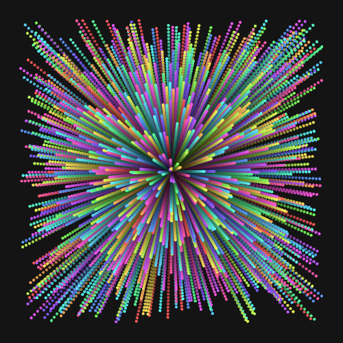
Recently I started making generative art with nannou.
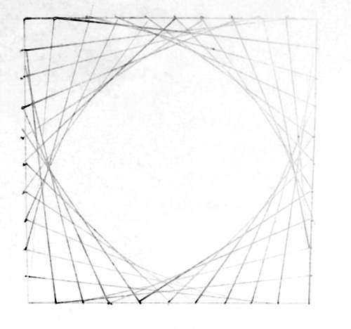
It made me think about when I first got interested. I can remember as a child in Primary school - 5- 11 year old - being tasked to make diagrams like this:
I can also remember in Year three - age eight - in art class and being given the project of filling an A4 page of square boxes with different patterns and being one of the few in the class to have finished the project.
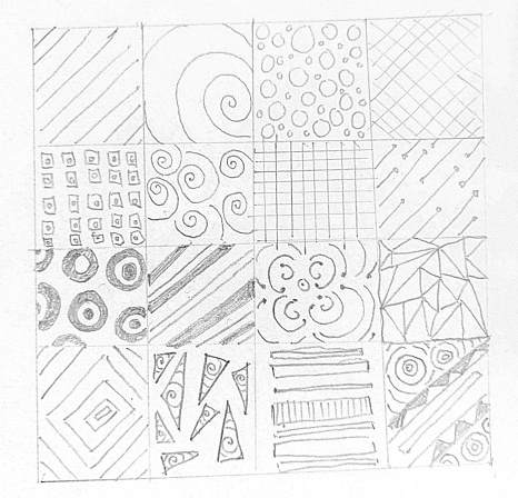
Doing it again now, I can see the appeal. There is something quite meditative about doing it. You have to think quite hard to avoid repeating ideas, but you're still only thinking about simple things.
As I got older I still enjoy the process, although now with code. During my PhD in number theory, I made some posters with the Reimann zeta function.
The first image is a plot of the Reimann zeta function along the half line for the first 100 zeroes. I imagine some people might recognise it. The second image is the fractional part of the imaginary part of the zeroes mapped to the unit circle. For my thesis I studied the the fractional part of the zeroes, which are uniformly distributed just like uniform random numbers. Hence you can use the fractional parts of the zeroes as a random number source. The third image is again a plot of the fractional part of the zeroes using the imaginary part as the height.
Generally I think they just look cool!